这篇文章通过对 FIR 传递函数进行因式分解,得到一个很长的 FIR 的滤波器可以由多个二阶滤波器组成,为之后利用二阶滤波器的特性去设计 FIR Notch Filter 建立底层的数学认知。
¶ FIR传函因式分解
FIR Filter 的定义与理解如下
FIR filters have a Finite Impulse Response, duh! But there are times when this finiteness is just what you need. A filter with an impulse response that’s strictly finite in length has a limited amount of ‘memory.’ Changes in the input signal that occurred at a time earlier than “‘now’ minus the duration of the impulse response” cannot possibly contribute to the latest output sample. If the input stabilizes to a constant value, the output will become exactly constant after a period equal to the duration of the impulse response. In other words, the settling time is finite, and known exactly.
In contrast, the output of an IIR filter is, in principle at least, affected by conditions in the input signal arbitrarily far back in the past. The output can also continue to change for an indefinitely long period of time after the input has stabilized. In a standard quantized digital implementation, it’s actually quite difficult to say for certain when the output will stop varying. In fact, sometimes it never does completely settle down, but fusses around for ever in a pattern called a limit cycle.
下面这句话很有意思,焦糖化反应和美拉德反应是厨师做菜的底层原理;数学/物理是工程师做项目的底层原理。问题来了,作为厨师,到底需要多大程度上理解这两个化学过程呢?
he good news is that you don’t need to be a filter expert or a math nerd to make progress here. For example, as a chef (to push that cooking metaphor), you can exploit the Maillard reaction to make tasty dishes, without needing to understand its chemistry. Likewise, you can play around with some algebra to create cool filters even if you’re not entirely comfortable with what it really means (yet…).
回归到正题,对于下面这个 FIR 的传递函数
首先观察这个这个 FIR 的幅频响应,具体做法是将 代入,假设 ,求其 范围内求
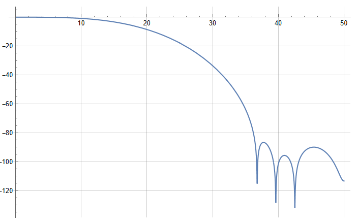
上面这个表达式,是一个一元14次方程,为了方便,这里将 替换为 (在 #理解延迟运算符z -1 会解释这样做的合理性),去求解 时 的解(利用 Mathematica 或者 Matlab),可以得到如下结果。其中4个是实数根(只有实部),10个复根(其实时5对共轭复根,实部相同,虚部相反)。
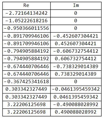
这里我们来回顾下高中数学,一个共轭复根的来源,对于一个存在共轭复根解的表达式,展开后得到
我们可以看到,如果求解 对 的解时,会得到一对 的 Complex Roots;这样我们就可以利用 Mathematica 求到解,直接写出表达式(1)的因式分解结果: 的系数是1, 的系数是 , 的系数
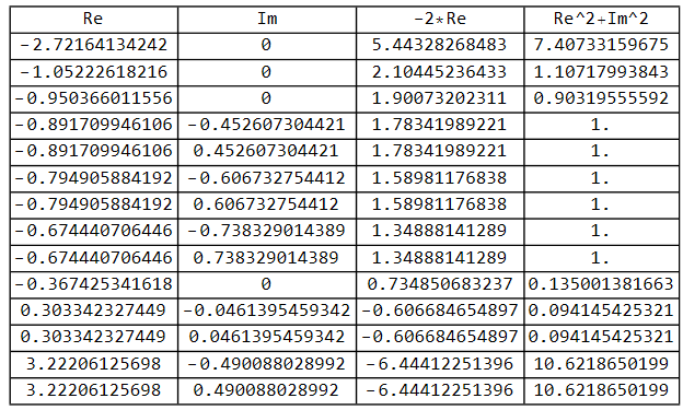
这个因式分解的结果,频域乘积代表着时域卷积,其实也就是系统的级联,从这个表达式中可以看到一个很长的 FIR 的滤波器可以由多个 二阶滤波器(3抽头) 或者 一阶滤波器(2抽头) 组成
My main goal is not to get you breaking down someone else’s FIR filter design using these tools, not yet anyway. What’s really interesting is to look at the behavior that the factors themselves exhibit. We can then separately manipulate each factor to potentially make it do something we want. If we create some factors from scratch, each of which does something useful and interesting, and then multiply them all up to get a polynomial, then this polynomial’s coefficients are those of an FIR filter that does all those interesting things at once.
我们发现在表达式(2)中,有三个二阶系统的 0 次项为 1(表达式第二行),然后观察到幅频响应中存在 3 个 Null 点,这并不是巧合。具体内容将在 Synthesize-FIR-Notch-Filters-By-Cascade-2nd-Order-FIRs 中详细解释并应用。
¶ 理解延迟运算符z^-1
Z-Transform , 表示延迟,如果在离散时域系统中进行如下操作(因果系统,只能对已经发生的事件处理)
其 Z-Transform 如下(Z-Transform 主要为了计算方便,其用于分析和处理离散信号系统,历史上出现的时间甚至早于傅里叶变换,后来欧拉公式将两种变换统一了起来,所以这里的算子,我们就单纯地将其当成一个人为定义的运算符号即可,至于后续在频域上的分析,我们当成一个分析工具或者分析模型即可,赋予物理意义追求直观理解,或许有益,或许只是一厢情愿)
这里为了计算方便,将 替换为了 ,这并不会影响幅频响应,因为复指数欧拉公式分解后,模 magnitude 是不变的
¶ Mathematica 计算代码
ClearAll["Global`*"]

(*定义系数列表*)
h = {+0.000427485, +0.001181126, -0.005110383, -0.023124099, \
-0.01358223, +0.091848493, +0.268171549, +0.359999657, +0.268171549, \
+0.091848493, -0.01358223, -0.023124099, -0.005110383, +0.001181126,
   0 + .000427485};

(*生成FIR传递函数 H(z)*)
Hz = Sum[h[[k + 1]] z^-k, {k, 0, Length[h] - 1}];

(* 替换z^-1 -> z, 这个只是为了简化运算 *)
Hz2 = Hz /. z -> 1/z;

(* 求解z^-1的根 *)
roots = Solve[Hz2 == 0, z];

(*表格打印*)
vals = z /. roots;
table = {Re[#], Im[#]} & /@ vals;
Grid[Prepend[table, {"Re", "Im"}], Frame -> All]
table = {Re[#], Im[#], -2*Re[#], Re[#]^2 + Im[#]^2} & /@ vals;
Grid[Prepend[table, {"Re", "Im", "-2*Re", "Re^2+Im^2"}], Frame -> All]

Hf = Hz /. z -> Exp[I*2*Pi*f];
Plot[20*Log10[Abs[Hf]], {f, 0, 0.5/1}]
¶ 参考资料
[[http://www.ednasia.com/analyze-fir-filters-using-high-school-algebra/]]